Shape-Bayes
Bayesian Inference of Structured Shapes under Visual Ambiguity
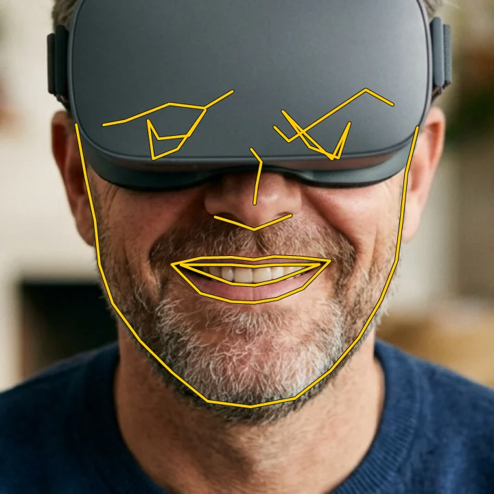
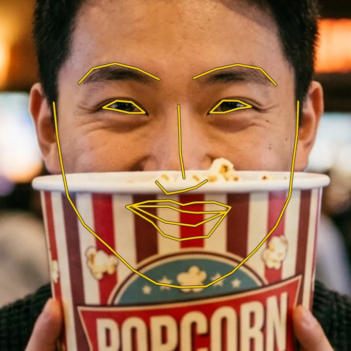
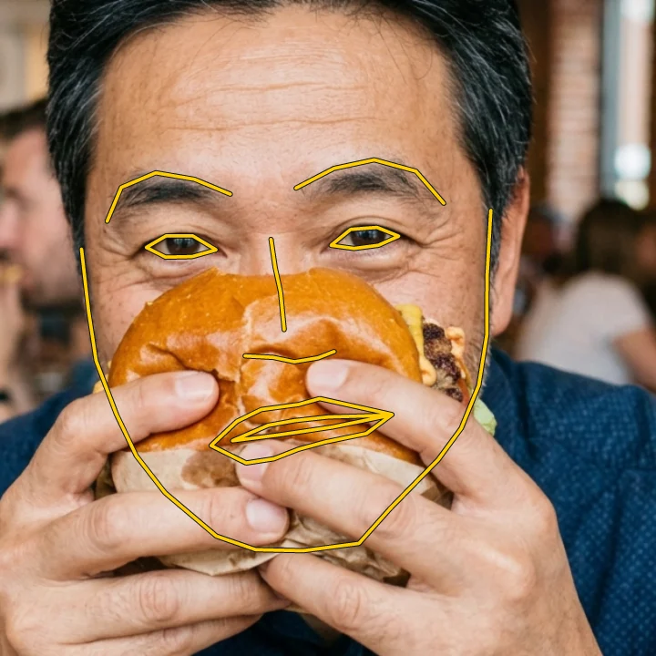
Trust visual evidence where it is reliable. Rely on the shape prior where it is ambiguous.The core intuition of Shape-Bayes
Abstract
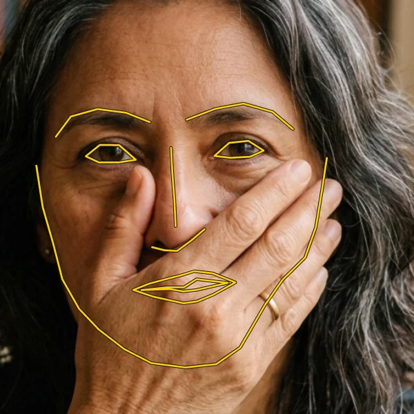
Perceiving structured shapes, such as human faces, from pixels is an inherently ambiguous task in real-world conditions. Yet shape inference is largely posed as a deterministic regression task predicting fixed spatial coordinates. We find that deterministic regression is brittle when visual evidence is ambiguous or incomplete: under severe occlusions, deterministic models exhibit structural collapse, predicting incoherent shapes or reverting to generic averages.
To address this, we introduce Shape-Bayes, a probabilistic framework that couples uncertainty-aware visual perception with Bayesian shape reasoning. Rather than forcing point estimates, Shape-Bayes dynamically weights visual evidence against geometric priors to infer a structurally valid shape posterior. By guaranteeing complete structural integrity, Shape-Bayes achieves 100% In-Distribution Rate (IDR) and establishes a new state of the art for robust 2D face shape regression under severe occlusion.
Structural Collapse Under Severe Occlusion
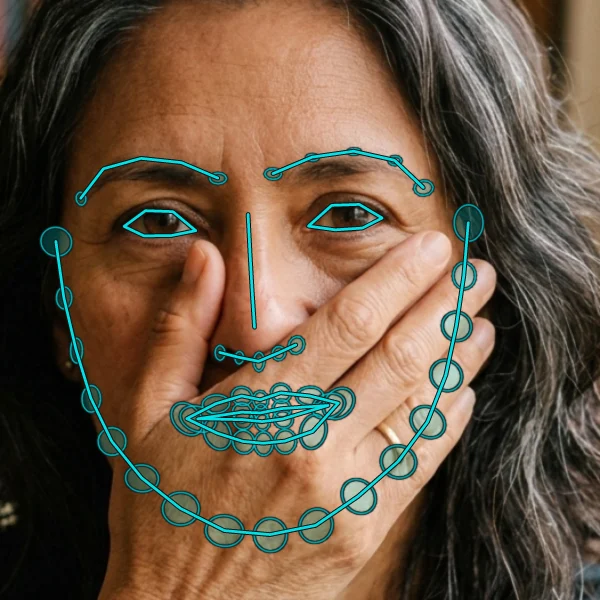
Deep regressors are highly accurate on unoccluded faces. But when a region has no meaningful visual evidence, a model that must output one point per landmark still has to guess. It either draws a topologically invalid shape or falls back to a generic average. Even HR-noSA, the state-of-the-art deterministic face shape regressor (Yang & Yeh, ICCV 2025), keeps only 66.6% of its 300W predictions inside the valid shape space once faces are occluded.
Even when its guess is plausible, a deterministic model gives one answer where the image supports several, and nothing tells the user that the answer was a guess.
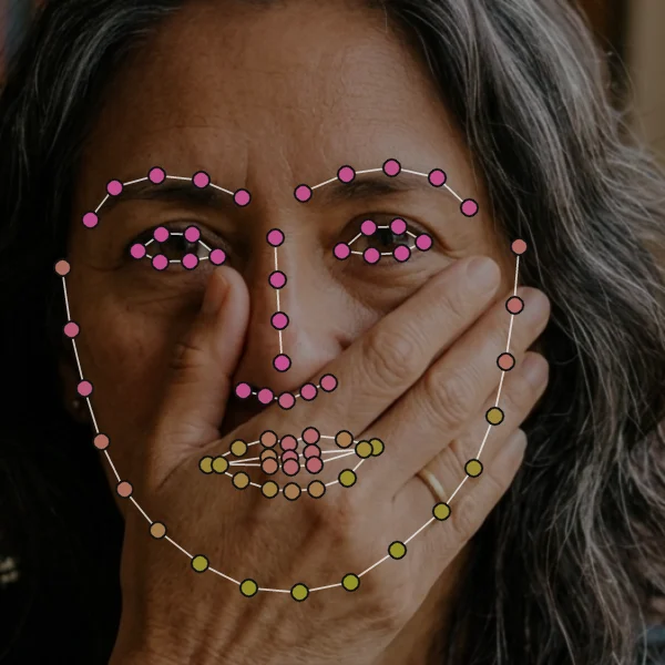
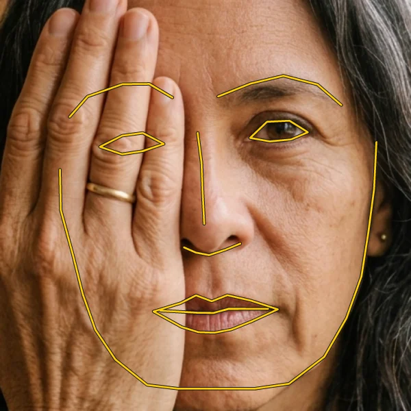
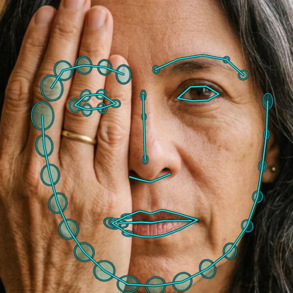
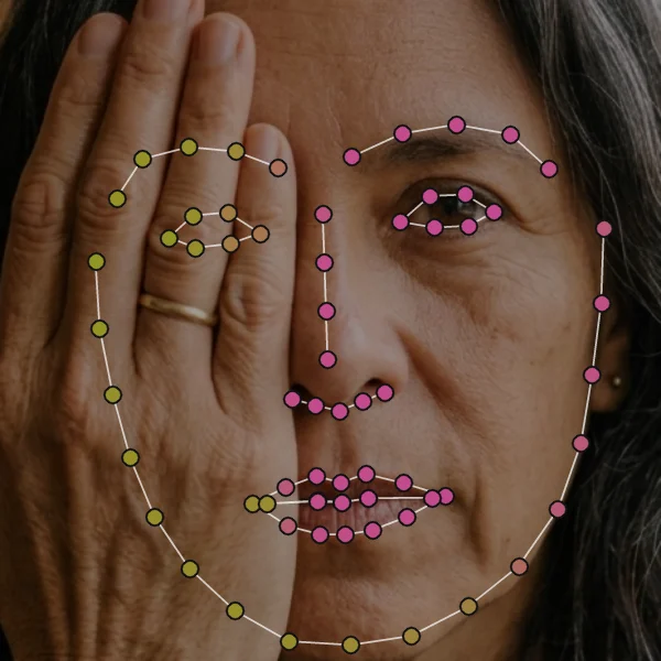
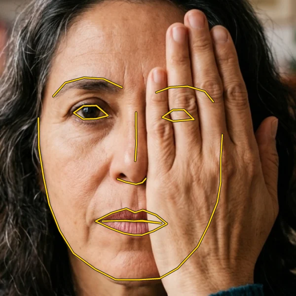
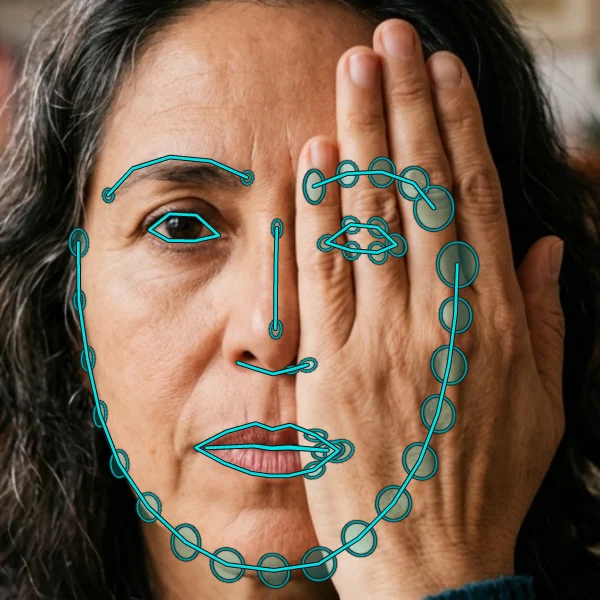
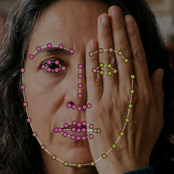
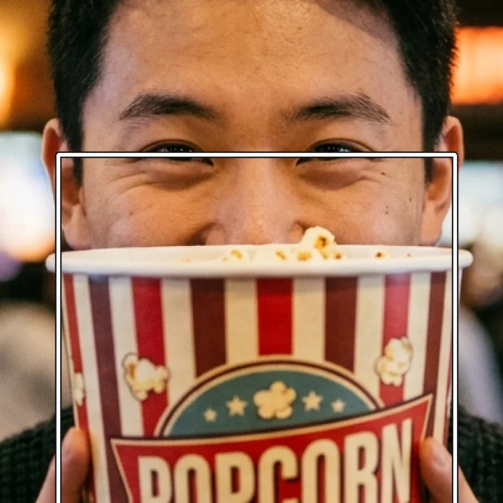
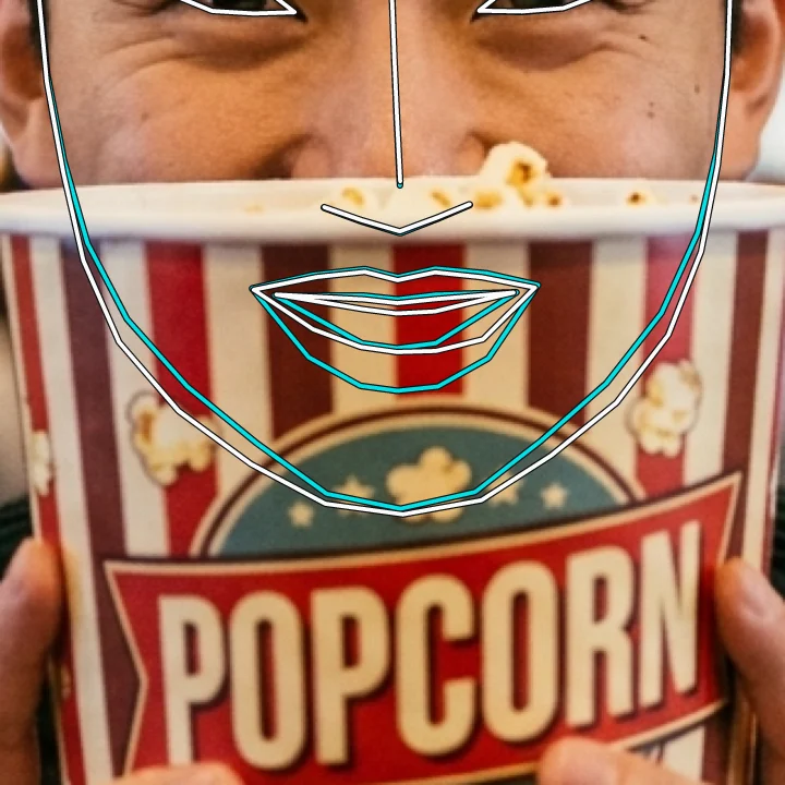
Drag the dividers to compare the same images: the deterministic base model on the left, the Shape-Bayes posterior with its uncertainty on the right.
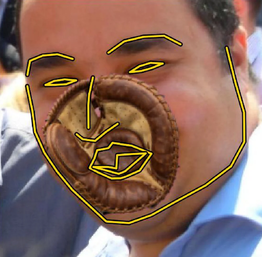
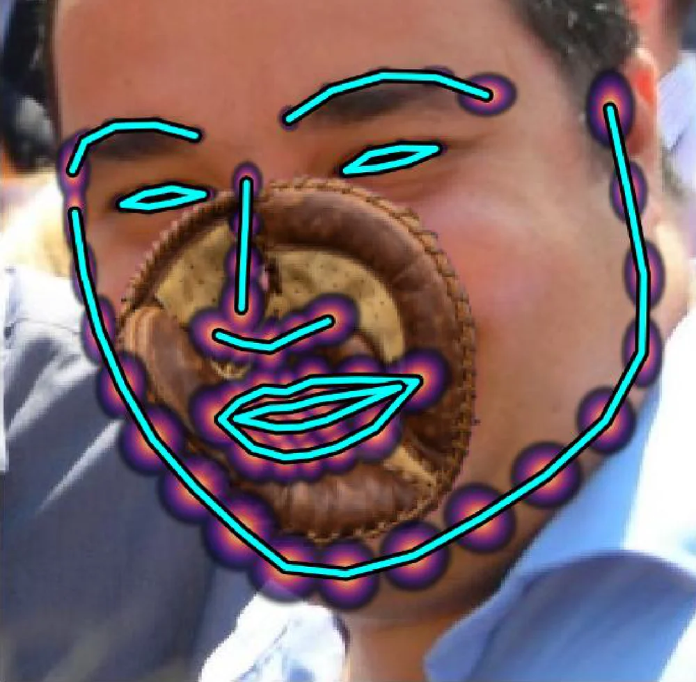
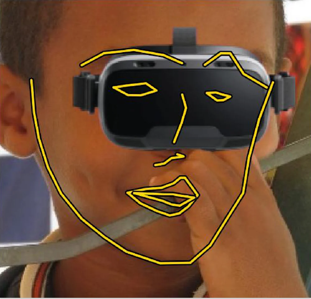
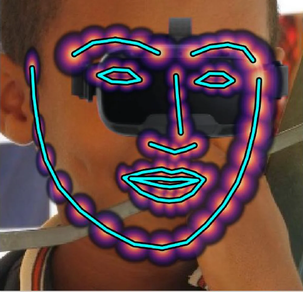
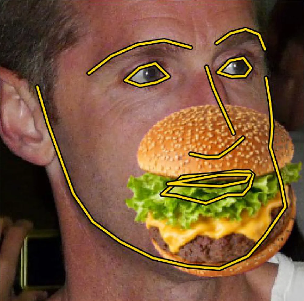
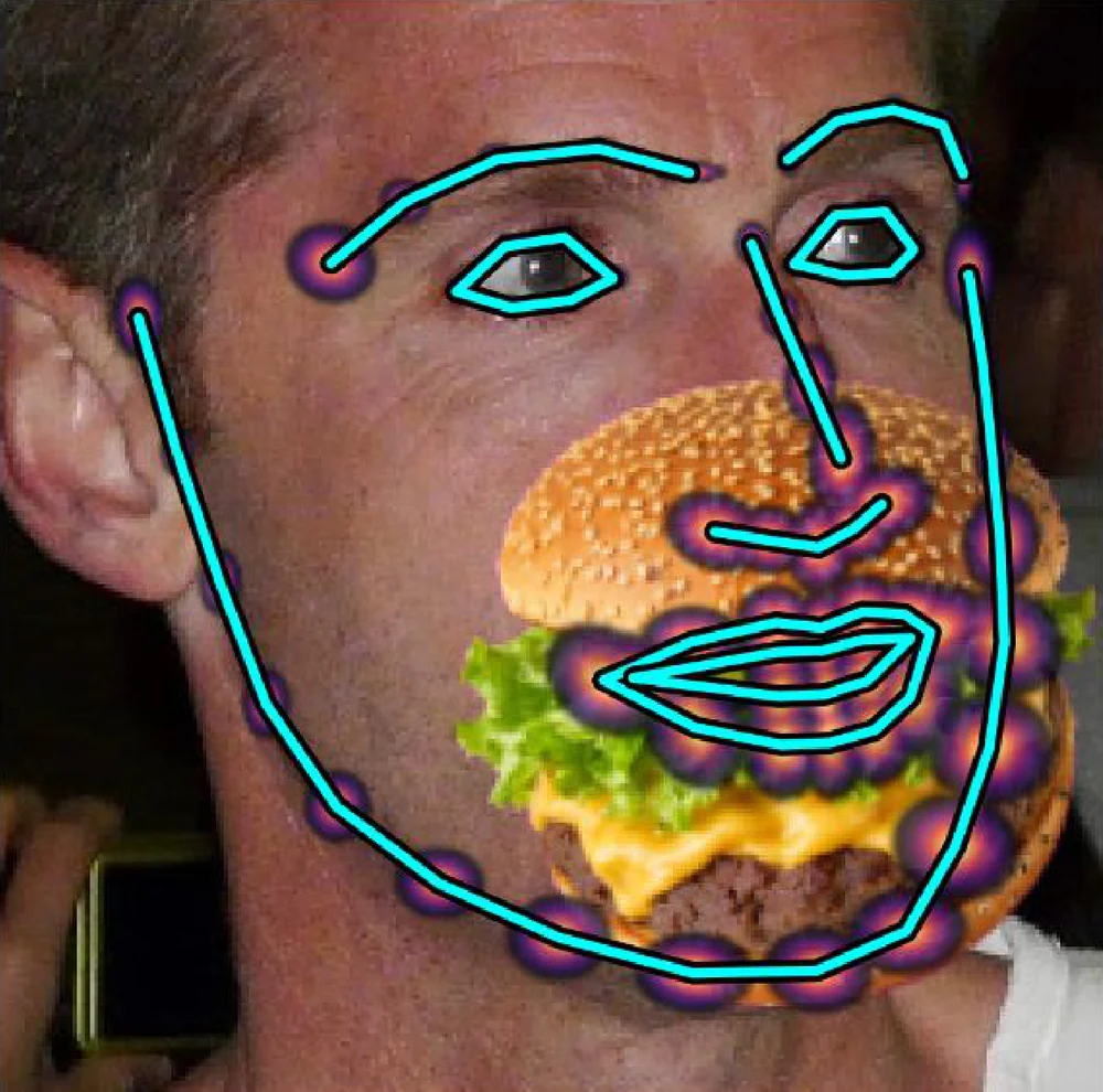
Occluded 300W test images. Left of each divider: HR-noSA (Yang & Yeh, 2025). Right: the Shape-Bayes posterior mean with per-landmark uncertainty.
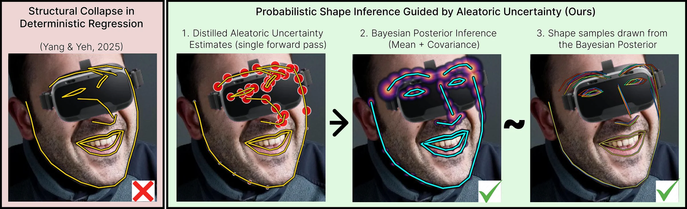
Adaptive Arbitration of Visual Evidence and Geometric Prior
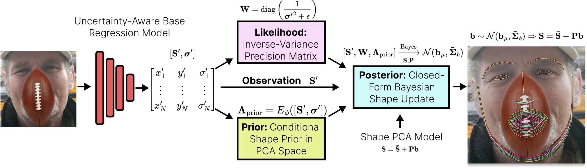
Human vision has long been described as Bayesian inference: incomplete, noisy bottom-up observations are reconciled with robust top-down structural priors. Shape-Bayes makes this explicit for shape regression. A base model reports not just where each landmark is, but how sure it is. We measure this "aleatoric uncertainty" intuitively: if an image is rotated or blurred and the model's prediction scatters, the model is uncertain. This distilled uncertainty acts as a spatial gate in a closed-form Bayesian update, deciding how much each coordinate can move the shape.
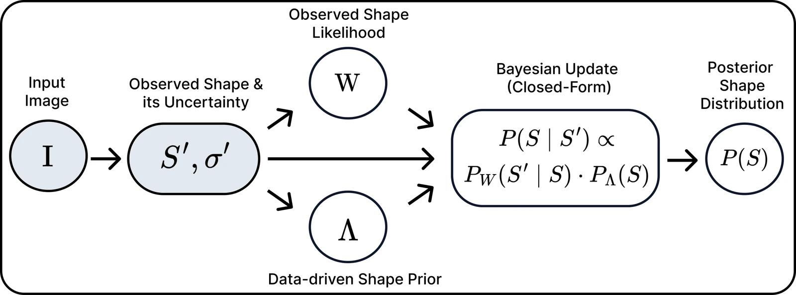
Posterior precision is a sum of information
Shapes live on a PCA manifold, \(\mathbf{S} = \bar{\mathbf{S}} + \mathbf{P}\mathbf{b}\). With a Gaussian likelihood and a Gaussian prior over the coefficients \(\mathbf{b}\), the posterior is exactly Gaussian. Its precision is the information from the image plus the information from the prior.
Where the face is hidden
\(\sigma' \to \infty\), so \(\mathbf{W} \to 0\). The observation term contributes no information there, and those landmarks are determined by the prior together with the visible landmarks. The estimate remains on the PCA shape manifold by construction.
Where the face is visible
\(\sigma' \to 0\), so \(\mathbf{W}\) dominates. Shape-Bayes becomes almost an identity mapping, so accuracy is kept: 300W NME goes from 2.86 to 2.81 on clean images.
Probabilistic Posterior Sampling
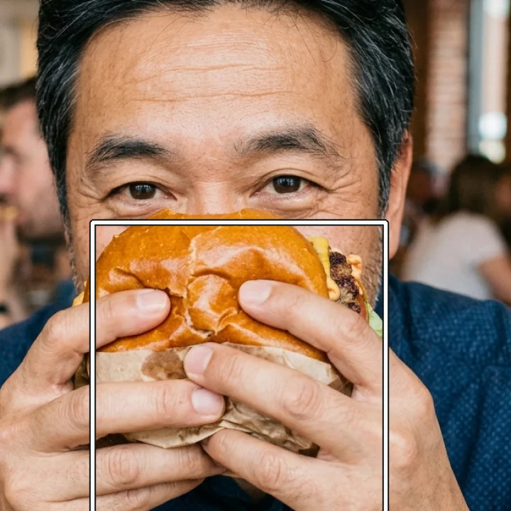
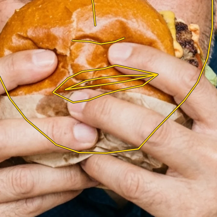
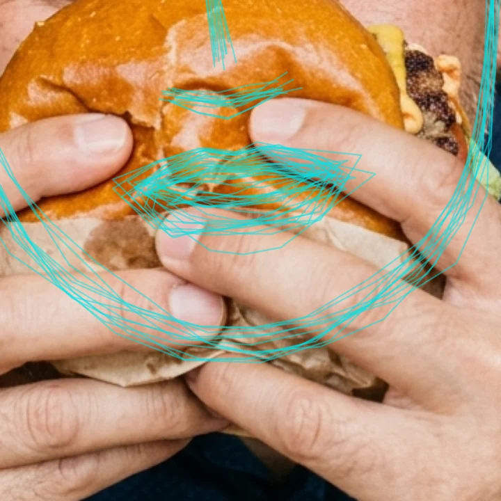
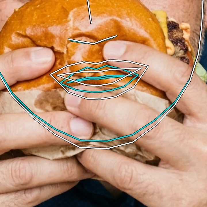
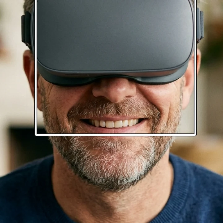
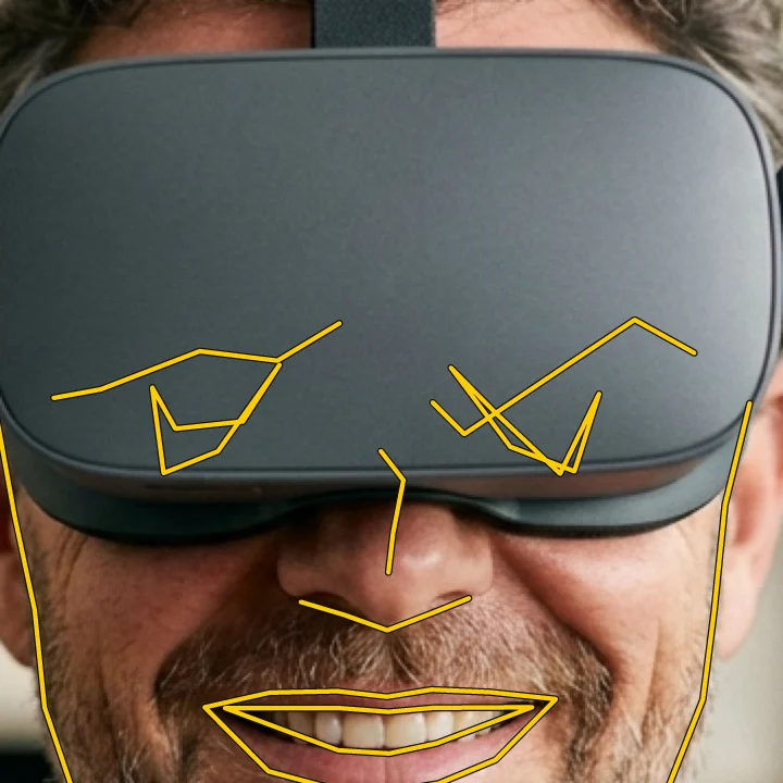
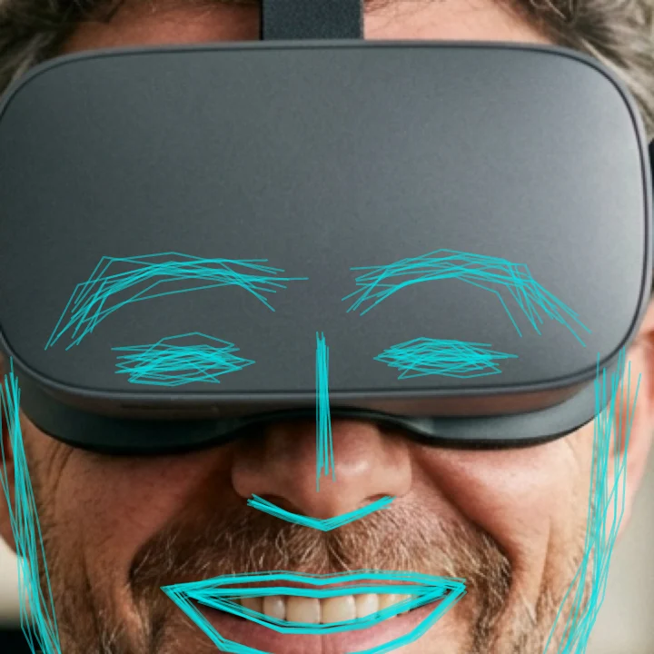
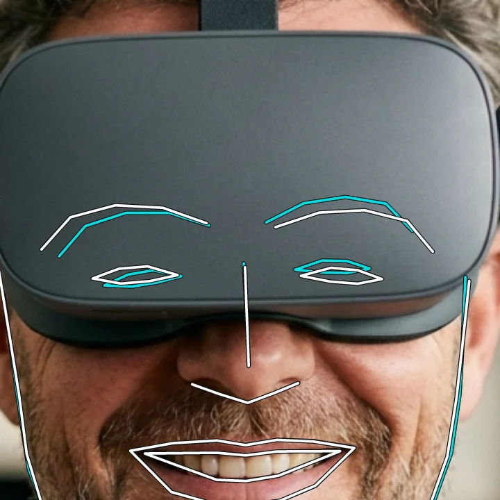
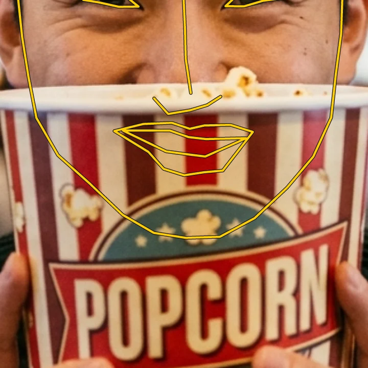
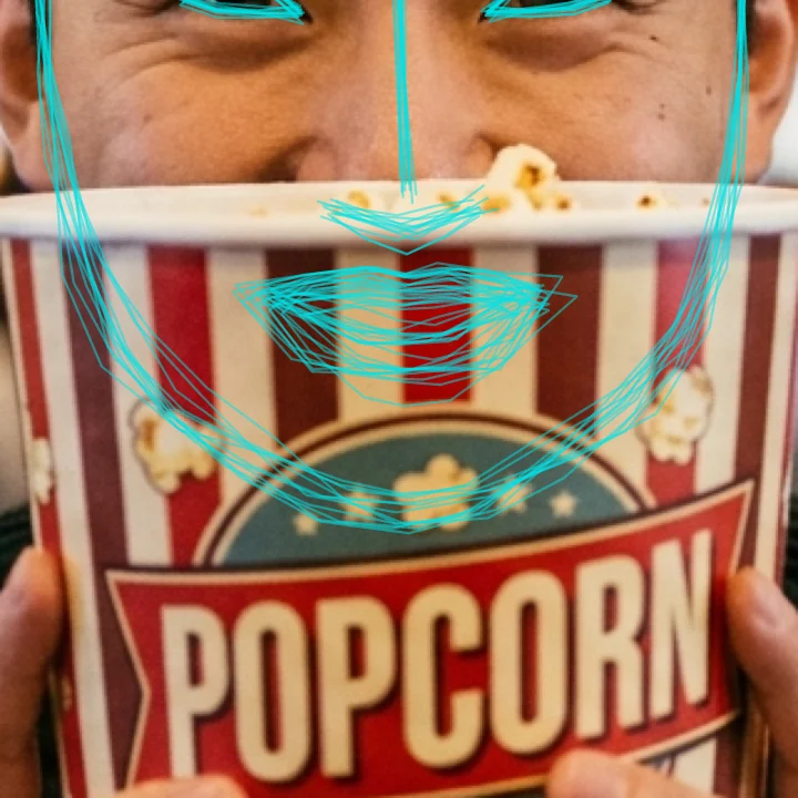
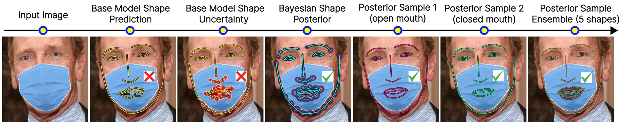
When an occluder covers a facial region, the visual evidence is insufficient to resolve ambiguities (e.g., whether the mouth is open or closed). A deterministic regressor still outputs a single shape with no measure of its reliability. In contrast, Shape-Bayes infers a closed-form Gaussian posterior over the PCA shape coefficients. Its principal directions of variance align with the unobserved shape dimensions: moving along the leading direction opens and closes the hidden mouth while the visible eyes stay fixed.
Posterior samples improve geometric accuracy
On occluded 300W, the posterior sample closest to the ground truth among 100 has an error of 6.60, against 9.03 for the deterministic prediction and 7.91 for the posterior mean. The minimum keeps decreasing with the number of samples, to below 6 at 1,000 (Fig. 9). Because selection uses the ground truth, this measures the quality of the hypothesis set, not of a deployable estimator. Realising the gain requires an external signal that discriminates between hypotheses, such as later video frames, a second view or a task-specific verifier.
Error on hidden landmarks (NME) ↓
Occluded 300W, HR-noSA base model. Best-of-N picks the sample using the ground truth, so it measures how good the hypothesis set is.
Three components, one exact update
Uncertainty from visual feature stability
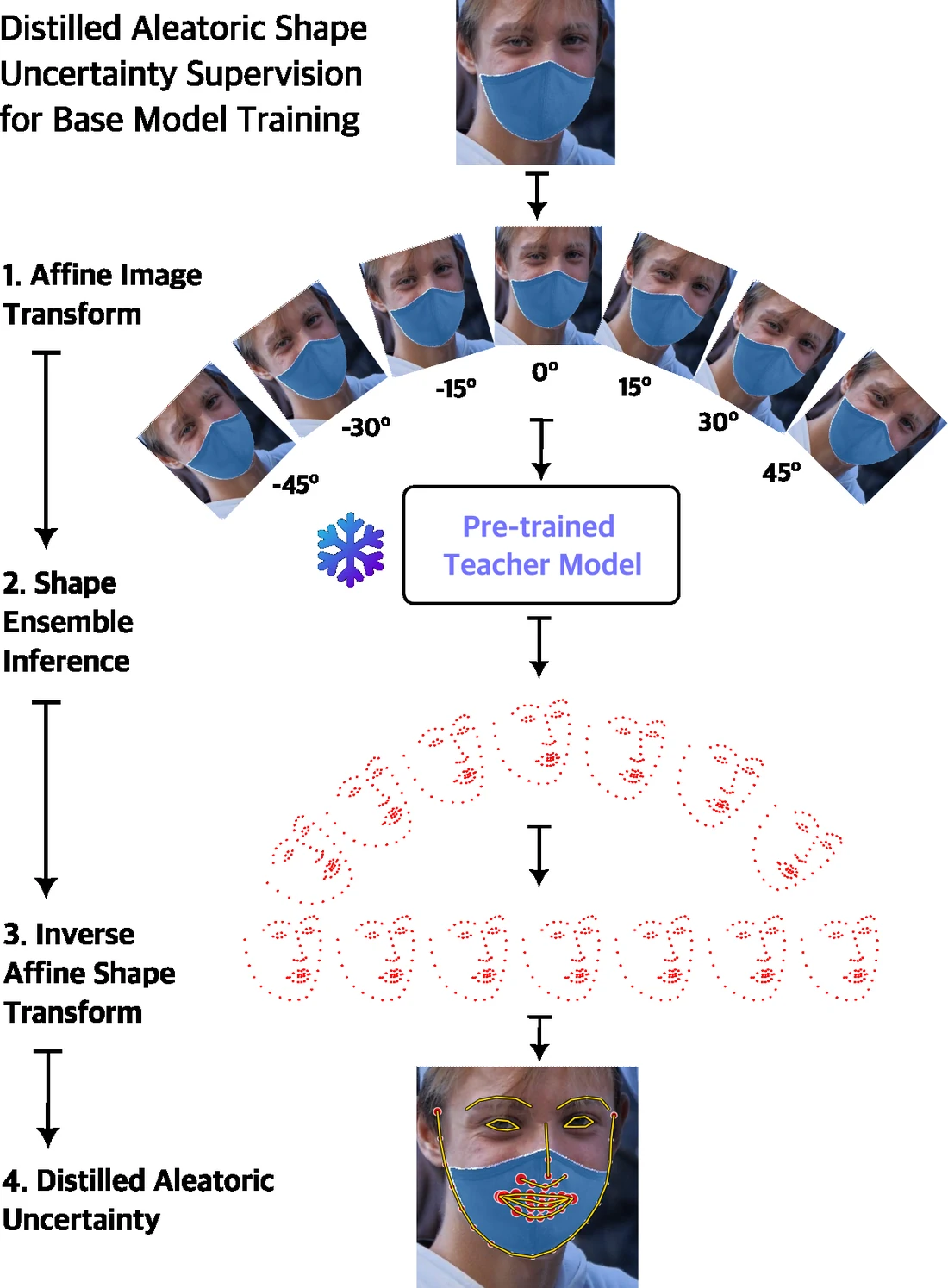
A visible, salient region has robust local features: its predicted coordinates barely move when the image is rotated, scaled or blurred. An occluded region has no discriminative evidence, so the model extrapolates from weak global context, and those guesses scatter under the same transformations.
Shape-Bayes turns this into supervision without manual labels. A frozen teacher predicts shapes for M augmented views. The predictions are warped back with the inverse transforms, and their root-mean-square deviation from the unaugmented prediction becomes the target uncertainty:
The base model learns to output coordinates and uncertainties together, so at inference it needs a single forward pass. The scheme works with any architecture: heatmap, coordinate or Transformer regressors. Models that already predict uncertainty, such as LUVLi, need no distillation at all.
Input-conditioned structural prior
A static PCA prior is often insufficient for large deformations such as head pose. Shape-Bayes employs a lightweight Transformer encoder conditioned on the observations: each of the N landmarks acts as a token, \(\mathbf{X} = [\mathbf{S}', \boldsymbol{\sigma}'] \in \mathbb{R}^{N\times 4}\).
Through self-attention, high-confidence visible regions inform the structural placement of occluded landmarks. The encoder outputs the diagonal of the prior precision matrix over the latent shape coefficients:
Prior \(\mathcal{N}(\mathbf{0},\, \boldsymbol{\Lambda}_{\text{prior}}^{-1})\) over \(\mathbf{b}\). The exponential keeps it strictly positive.
Differentiable closed-form Bayesian solver
The product of the likelihood and prior yields an exact Gaussian posterior over shape coefficients. Because the PCA manifold is low-dimensional, inverting the K×K precision matrix is computationally trivial and fully differentiable, enabling end-to-end training.
The posterior mean serves as the nominal shape prediction, while samples drawn from the posterior represent plausible alternative hypotheses. By construction, every sample lies on the valid PCA shape manifold.
Decoupling spatial prediction and uncertainty
During training, the base model is frozen and the PCA basis is precomputed; only the prior Transformer is optimized using occlusion-augmented shapes. An MSE objective on the posterior mean anchors the spatial coordinates, while a negative log-likelihood (NLL) objective calibrates the posterior.
A stop-gradient applied to the mean within the NLL term decouples these objectives: MSE governs spatial localization, while NLL governs uncertainty estimation. This prevents the model from artificially reducing the NLL loss by shifting the mean rather than properly calibrating its variance.
\(\bar{\mathbf{b}}_{\mu} = \operatorname{sg}[\mathbf{b}_{\mu}]\) is a stop-gradient on the mean.
Structural Validity and Occlusion Robustness
Shape-Bayes is evaluated on the 300W, WFLW and COFW test sets under a dynamic occlusion protocol: synthetic wearable masks and a library of more than 80 real-world objects overlaid on the images, without changing the ground-truth shapes. It is attached to six state-of-the-art base models spanning heatmap, coordinate and Transformer paradigms.
In-distribution rate (IDR) ↑
% of predicted shapes inside the 95% hyperellipsoid of the shape manifold
Error on occluded landmarks (NMEocc) ↓
Normalized mean error, % of inter-ocular distance
| Base model | IDR ↑ | NMEocc ↓ | NMEall ↓ | minNME@100 ↓ | FR10 ↓ | AUC10 ↑ |
|---|
Each cell shows base → +Shape-Bayes, with the relative change for error metrics. NATIVE marks models that already output uncertainty and need no distillation. A dash means the model was not evaluated on that benchmark. minNME@100 takes the posterior sample closest to the ground truth out of 100, so it measures the quality of the hypothesis set rather than of a single prediction.
Preserving structural integrity without over-smoothing
Prior-driven shape regularization typically trades accuracy on visible landmarks for global structural validity. Shape-Bayes avoids this trade-off. High-confidence visible landmarks strongly anchor the latent shape, while uncertain landmarks are down-weighted and inferred via the structural prior.
These gains are not traded between regions: on occluded 300W, error decreases across all facial parts.
Part-wise NMEocc on occluded 300W ↓
Base model: HR-noSA
Performance on unoccluded test sets
In the absence of occlusion, predicted uncertainties approach zero, causing the observation precision to dominate the prior. Shape-Bayes naturally reduces to an identity mapping, preserving or slightly improving baseline accuracy. Sampling 100 shapes from the posterior and selecting the oracle minimum yields the lowest error across all three benchmarks, confirming that the posterior assigns high probability mass to accurate geometric hypotheses.
| Method | 300W | WFLW | COFW |
|---|---|---|---|
| AWing | 3.07 | 4.36 | 4.94 |
| LUVLi | 3.23 | 4.37 | – |
| ViTPose | 3.02 | 4.26 | 4.85 |
| ADNet | 2.93 | 4.14 | 4.68 |
| HIH | 3.09 | 4.08 | 4.63 |
| SLPT | 3.17 | 4.14 | 4.79 |
| STAR | 2.90 | 4.03 | 4.62 |
| OccFace | 2.83 | 3.77 | 4.53 |
| HR-noSA | 2.86 | 3.97 | 4.53 |
| + Shape-Bayes (mean) | 2.81 | 3.94 | 4.50 |
| + Shape-Bayes (minNME@100) | 2.79 | 3.72 | 4.23 |
NMEall ↓ on the original test sets. Bold marks the best single prediction per benchmark. The minNME row selects among samples using the ground truth and is reported separately.
Ablation study
| Configuration | NME ↓ | minNME@100 ↓ | FR ↓ | AUC ↑ |
|---|
Unweighted least-squares PCA projection yields minimal improvement, as corrupted landmarks act as outliers that distort confident predictions. Weighting the projection by the distilled inverse variance—equivalent to Mahalanobis distance minimization—provides the majority of the performance gain. The adaptive prior accounts for the remaining improvement by accommodating input-specific variations such as head pose.
Because the output is a full probability distribution, drawing additional samples increasingly yields more accurate geometric hypotheses, significantly outperforming the deterministic baseline.
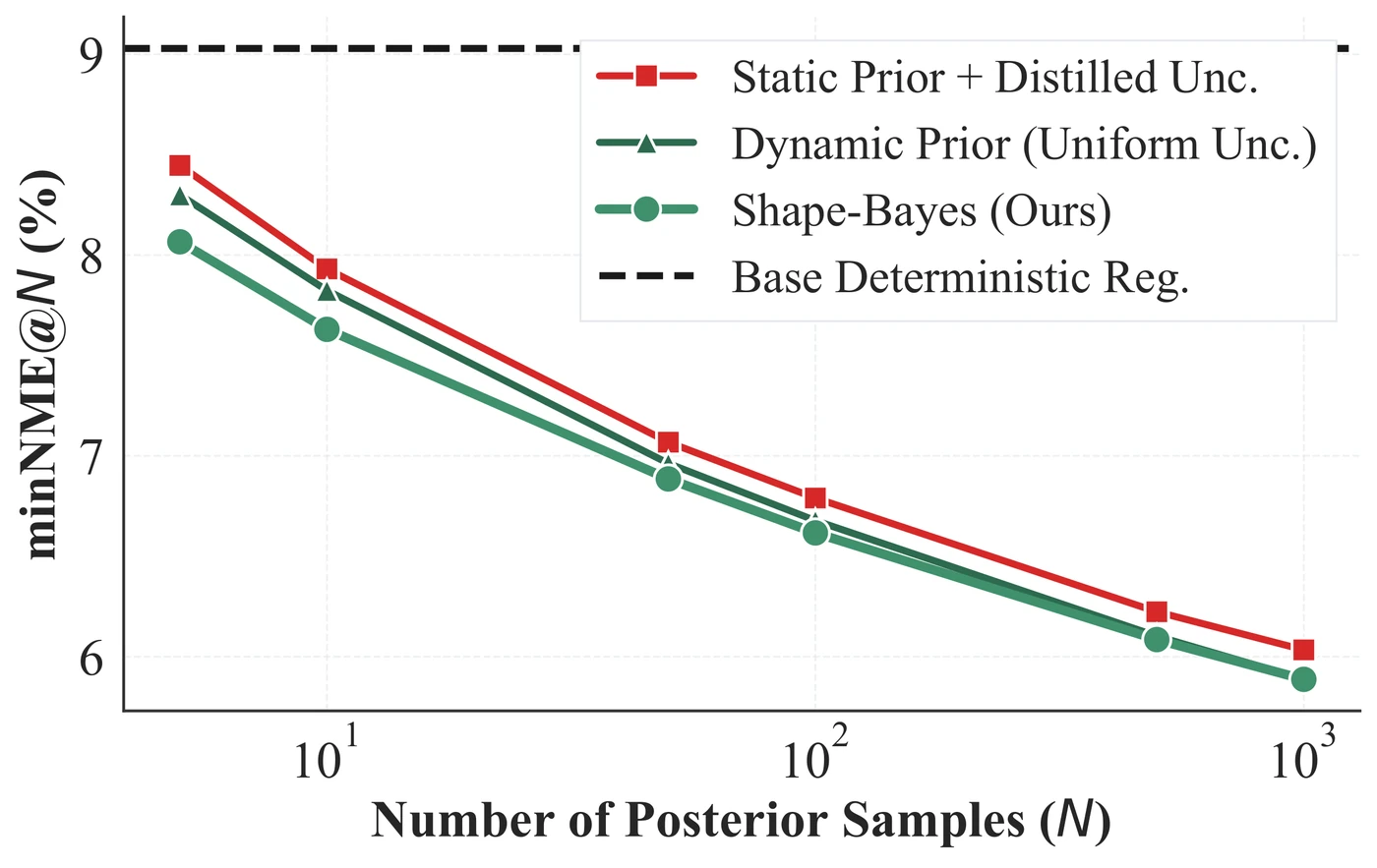
Occluded 300W, HR-noSA base model, metrics on occluded landmarks.
Posterior calibration
Under out-of-distribution occlusion, baseline models are typically overconfident, predicting uncertainties that underestimate the true error. Propagating aleatoric uncertainty through the prior-constrained Bayesian update appropriately increases the posterior variance where visual evidence is degraded, consistently lowering the expected calibration error (ECE) across all evaluated architectures.
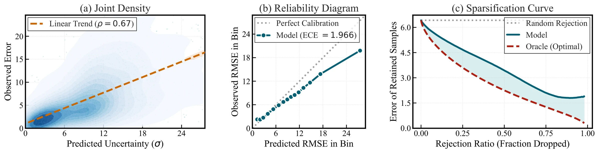
Expected calibration error (ECE) ↓
Occluded 300W. *LUVLi uses its own native uncertainty.
| Base model | NLL ↓ | ECE ↓ |
|---|
Qualitative results across benchmarks
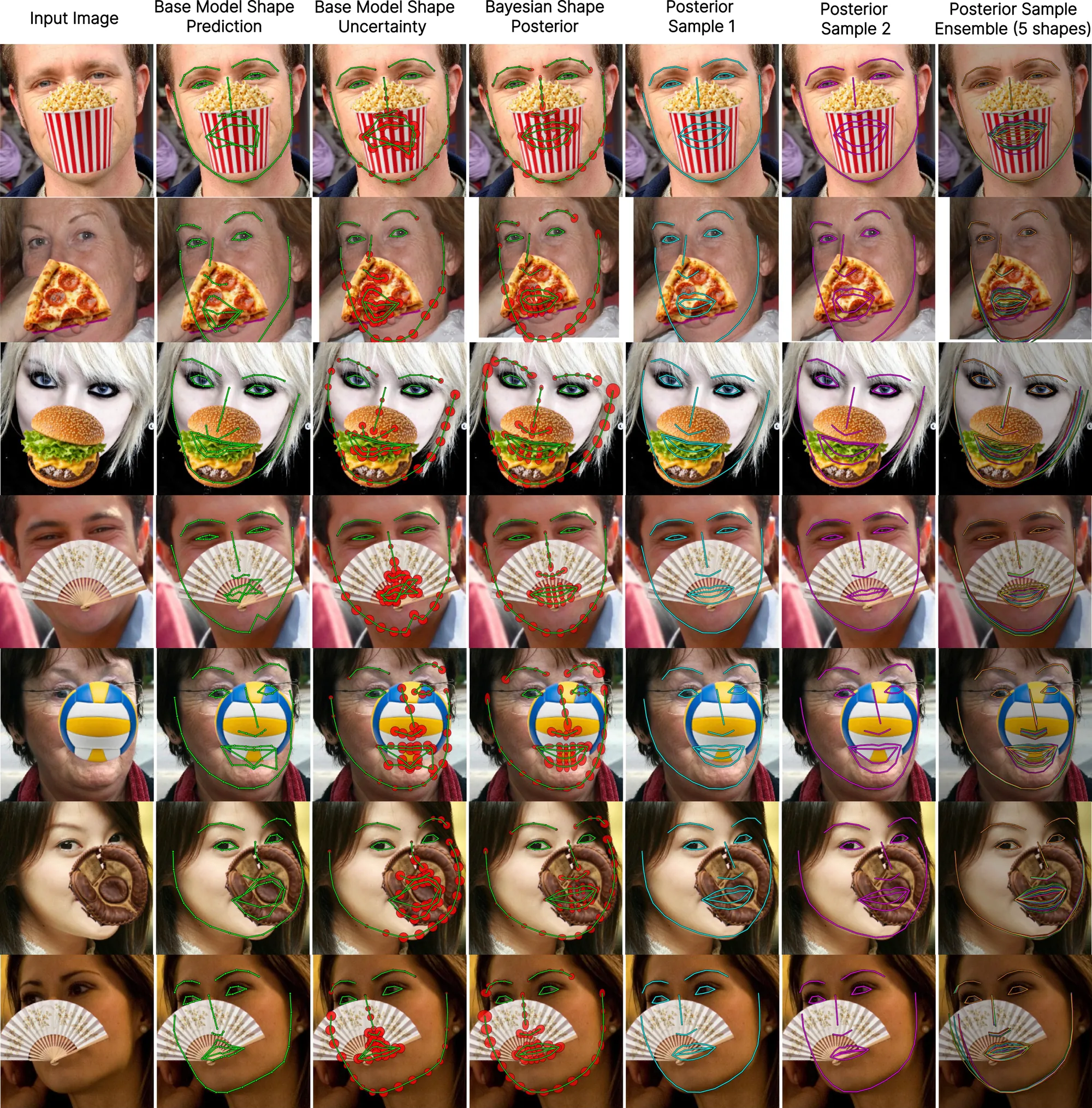
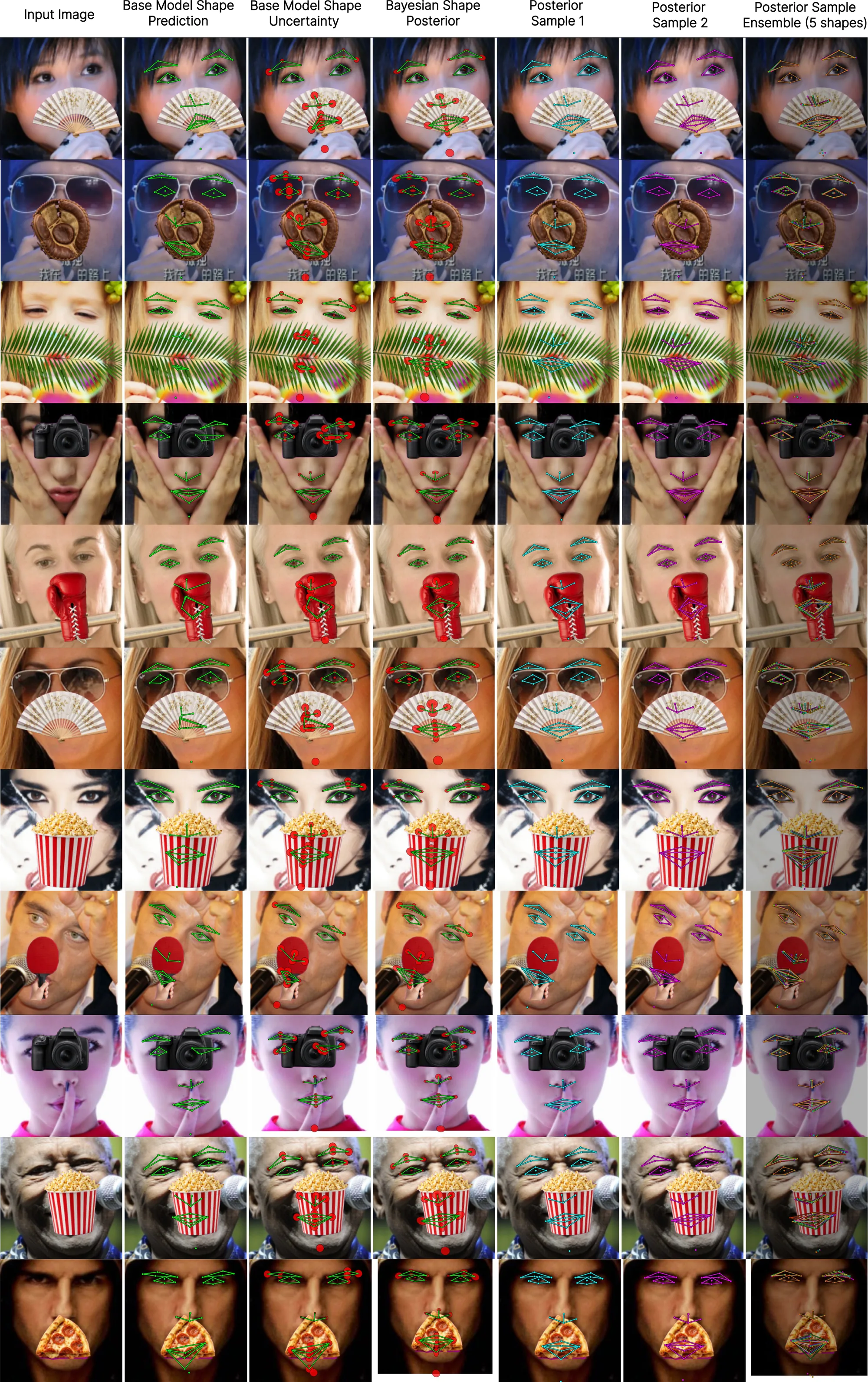
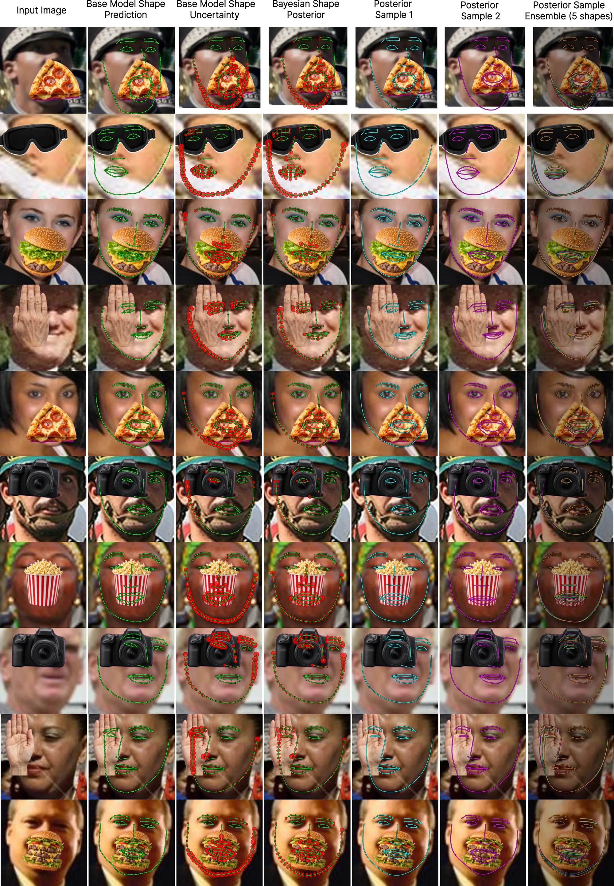
HR-noSA (Yang & Yeh, 2025) base model versus Shape-Bayes on dynamically occluded test images.
Computational cost
As the base network remains frozen, Shape-Bayes introduces only a lightweight Transformer and a K×K matrix inversion. Consequently, the backbone continues to dominate total inference time.
Generalization to other topologies
While evaluated on human faces—characterized by extreme rigid and non-rigid deformations, strict anatomical constraints, and abundant occlusion—the proposed Bayesian solver is topology-agnostic. It requires only a set of landmarks, their associated uncertainties, and a shape basis.
The framework naturally extends to other structured shape inference tasks under ambiguity, such as body and hand pose estimation, medical anatomical landmarking, and lane geometry extraction.
BibTeX
@article{tellamekala2026shapebayes,
  title   = {Shape-Bayes: Bayesian Inference of Structured Shapes
             under Visual Ambiguity},
  author  = {Tellamekala, Mani Kumar and Brown, Tosh and Valstar, Michel},
  journal = {arXiv preprint arXiv:XXXX.XXXXX},
  year    = {2026}
}